Summary and Implementation of Particle Swarm Optimization

Posted on 2024-05-08 Edited on 2024-10-24 Views: Word count in article: 1.1k Reading time ≈ 4 mins.

Particle swarm optimization (PSO) was first proposed by James Kennedy and Russell Eberhart in 1995, also known as particle swarm algorithm.

The basic idea of the particle swarm algorithm comes from the study of the foraging behavior of bird flocks. Each particle can be regarded as a bird, and the process of searching for a solution is similar to the process of a flock of birds looking for food. In the process of searching for food, each bird knows the best location it has found. At the same time, information is shared within the flock, so that each bird also knows the best location the entire flock has found.

The advantage of PSO is that it is simple, easy to implement, has fewer parameters that need to be adjusted, and has better global optimization capabilities.

Basic Concept

The position of the $i$ -th particle: $X_i=(x_{i1},x_{i2},...,x_{iD})$

The velocity of the $i$ -th particle: $V_i=(v_{i1},v_{i2},...,v_{iD})$

Each particle has three properties: speed, position and fitness. The velocity represents the distance and direction of movement of the particles, and the position is the solution to the corresponding practical problem. The above formula gives the position and velocity of the particle including D-dimensional components. For example, for the function $f(x)=x+y$ , the position of a particle can be expressed as $(x, y).$ At this time, the speed and position of the particle are both 2-dimensional. Fitness is calculated by the fitness function and is used to evaluate the quality of a particle.

The particle swarm algorithm first needs to initialize a group of particles, randomly initialize the position and speed of each particle, and then search for the global optimal solution through continuous iteration. In each iteration, the particle updates its speed and position by tracking two "extreme values" (individual extreme value $P_{best}$ , group extreme value $G_{best}$ .

Velocity Update

v^{k+1}_{id}=\textcolor{blue}{\omega v^{k}_{id}}+\textcolor{Purple}{c_1r_1(p^{k}_{id}-x^{k}_{id})}+\textcolor{OrangeRed}{c_2r_2(g^{k}_{d}-x^{k}_{id})}

The relevant variables in the formula have the following meanings:

$v^{k+1}_{id}$ : The $d$ -dimensional velocity component of particle $i$ at the $k$ -th iteration

$x^{k}_{id}$ : The $d$ -dimensional position component of particle $i$ at the $k$ -th iteration

$\omega$ : Inertia factor ( $>0$ )

$c_1$ , $c_2$ : Learning factor}

$r_1$ , $r_2$ : Random numbers in the interval $(0, 1)$ to increase the randomness of the search

$p^{k}_{id}$ : The $d$ -dimensional position component of the individual extreme value $P^{i}_{best}$ of particle $i$ after the first $k$ iterations}

$g^{k}_{d}$ : The $d$ -dimensional position component of the population extreme value $G_{best}$ of the entire particle population after the first $k$ iterations

Inertia term: reflects the influence of the particle’s last velocity.

Self-cognition items: the particle’s own experience, the distance and direction between the particle’s current position and its historical optimal position.

Group cognition items: information sharing among all particles, the distance and direction between the current position of the particle and the historical optimal position in the population.

For each dimensional component of each particle's velocity, it needs to be updated according to this formula. It can be seen from this formula: Next movement direction of the particle $=$ Inertial movement direction $+$ Optimal movement direction recognized by itself $+$ Optimal movement direction recognized by the group.

Position Update

x^{k+1}_{id}=x^{k}_{id}+v^{k+1}_{id}

For each dimensional component of each particle's position, it needs to be updated according to this formula. The position of each particle is the solution to the actual problem, so the position update process of the particles is the search process for the solution. Every time the particle updates its position, it needs to calculate the fitness and update the individual extreme value $P_{best}$ and the group extreme value $G_{best}$ .

Parameter Settings

Particle swarm size

When the population size is small, the algorithm easily falls into local optimality, while when the population size is large, the search efficiency can be higher, but the amount of calculation in each iteration will also increase. Usually when the population size increases to a certain level, the effect of increasing the population size will be limited.

Inertia factor

Also called inertia weight, the larger the value, the stronger the particle's ability to explore new areas. A better approach is to let the algorithm conduct more random explorations in the early stages of the search, while in the later stages it is more likely to use existing experience. This idea is similar to the balance between exploration and exploitation in Reinforcement Learning (RL).

\omega=\omega_{max}-(\omega_{max}-\omega_{min}){i\over i_{max}}

The relevant variables in the formula have the following meanings:

$\omega_{max}$ : Maximum inertia weight

$\omega_{min}$ : Minimum inertia weight

$i$ : Current number of iterations

$i_{max}$ : Maximum number of iterations

Common adjustment strategies include linearly decreasing inertia weight: as the number of iterations increases, the inertia weight will continue to decrease, similar to the above formula.

Maximum speed of particles

If the speed of a particle exceeds the set maximum speed $V_{max} (>0)$ , the speed of the particle is set to $V_{max}$ . When $V_{max}$ is large, the particles fly fast and the algorithm has strong search ability, but it is easy to fly past the optimal solution. When $V_{max}$ is small, it is easy to fall into the local optimal solution.

Example

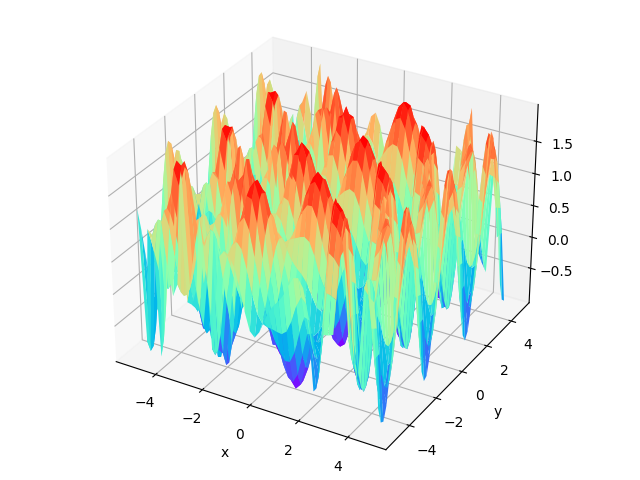
Objective Function

Next, we try to use PSO to find the maximum value of this function:

z=sin((1-x)^2+2y+cos(x^2))+sin(x+y)^2

The graph of the objective function is as follows:

Result

In the iterative process of the PSO algorithm, the fitness change process of the optimal solution found is as follows:

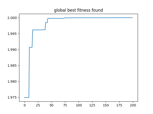
The optimal solution found by PSO is as follows:

1 2	The optimal (maximum) solution found: [1.02996889 0.54137418] The fitness of the found solution: 1.9999992081662792

Code

The Python code of the PSO is here: Optimization/metaheuristic_algorithms/Particle_Swarm_Optimization/PSO.py (github.com)

Reference Links

https://en.wikipedia.org/wiki/Particle_swarm_optimization